All Courses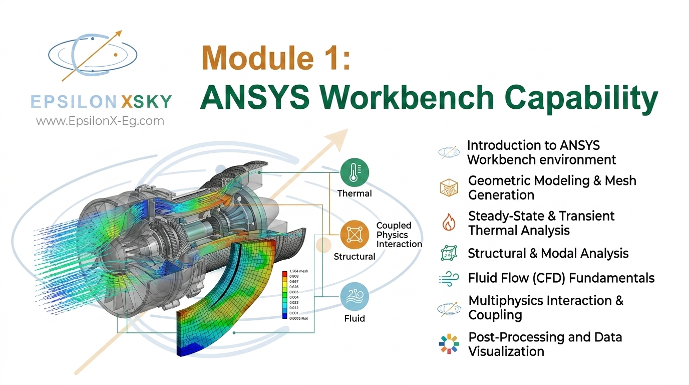
Course
Module 1: ANSYS Workbench Capability
7 sessions2 free previews
Curriculum
What you'll learn
7 sessions · 2 free
0127m0223m
ANSYS Capabilities, Workbench Ecosystem & Simulation Design Basis (Lecture One)
ANSYS Capabilities, Workbench Ecosystem & Simulation Design Basis (Lecture Two)
0317m
ANSYS Capabilities, Workbench Ecosystem & Simulation Design Basis (Lecture Three)
0423m
ANSYS Capabilities, Workbench Ecosystem & Simulation Design Basis (Lecture Four)
0529m
ANSYS Capabilities, Workbench Ecosystem & Simulation Design Basis (Lecture Five)
0629m
ANSYS Capabilities, Workbench Ecosystem & Simulation Design Basis (Lecture Six)
0718m
ANSYS Capabilities, Workbench Ecosystem & Simulation Design Basis (Lecture seven)
Overview
About this course
Module 1: ANSYS Workbench Capability
Understanding the ANSYS Ecosystem, Physics Selection & Engineering Simulation Workflows
Module 1 provides the foundation for the entire Industry-Oriented CAE Simulation MasterClass at Epsilon X Sky. The objective is to help engineers understand the ANSYS ecosystem, recognize the capabilities and limitations of different solvers, and confidently select the appropriate simulation approach for a given engineering problem.
Rather than focusing only on software operation, this module develops the engineering judgment required to answer a fundamental question:
Which physics, solver, and modeling approach should be used for this problem?
Introduction to ANSYS Workbench
The module begins with a comprehensive introduction to the ANSYS Workbench environment and its role as an integrated platform for engineering simulation.
Participants learn how different ANSYS systems can be connected within a common workflow, from initial geometry preparation through simulation, post-processing, and final engineering reporting.
The workflow is presented from an industrial perspective:
CAD → Geometry Preparation → Physics Selection → Meshing → Solver Setup → Solution → Post-Processing → Validation → Engineering Report
This provides participants with a clear understanding of how individual ANSYS tools fit into a complete CAE workflow.
Understanding the ANSYS Solver Ecosystem
A major component of the module is an overview of the principal ANSYS solvers and engineering platforms, including:
-ANSYS Mechanical – Structural and mechanical analysis.
-ANSYS Fluent – Advanced CFD, heat transfer, multiphase flow, combustion, and fluid-flow applications.
-ANSYS CFX – CFD applications with a strong focus on turbomachinery and complex fluid systems.
-ANSYS Polyflow – Specialized applications involving complex fluid behavior and polymer processing.
-ANSYS Discovery – Rapid simulation, design exploration, and interactive engineering analysis.
-ANSYS Icepak – Electronics cooling and thermal-management applications.
-ANSYS Sherlock – Electronics reliability and life-prediction applications.
-ANSYS SIwave – High-speed PCB and electromagnetic simulation.
-ANSYS HFSS – Introduction to high-frequency electromagnetic and antenna analysis.
Participants learn not only what each solver does, but also when it should and should not be used.
Solver Capabilities & Limitations
Selecting a solver correctly is one of the most important decisions in computational engineering.
This section helps participants understand:
-Solver capabilities
-Appropriate application areas
-Modeling assumptions
-Physics limitations
-Computational requirements
-Expected outputs
-Solver compatibility
Engineers learn to avoid the common mistake of selecting a solver simply because it is familiar, instead choosing the approach based on the actual physics of the engineering problem.
Coupled Physics & Multiphysics
Modern engineering systems frequently involve more than one physical phenomenon.
The module introduces the fundamentals of multiphysics simulation, including:
One-Way Coupling
Information is transferred from one physics domain to another without significant feedback from the receiving system.
Two-Way Coupling
The physical systems interact with each other, with information exchanged in both directions during the simulation.
System Coupling
Participants are introduced to the concept of connecting different ANSYS solvers to simulate complex interacting physical systems.
Applications may involve combinations such as:
-CFD + FEA → Fluid–Structure Interaction
-CFD + Thermal → Conjugate Heat Transfer
-Structural + Thermal → Thermomechanical Analysis
-Electromagnetics + Thermal → Electromagnetic Thermal Management
This section establishes the foundation for the advanced multiphysics projects covered later in the course.
1D, 2D & 3D Engineering Modeling
Participants explore the different approaches used to represent engineering systems numerically.
1D Modeling
Using line elements and simplified representations for applications such as:
-Beams
-Trusses
-Piping
-Structural networks
2D Modeling
Using shell or planar representations where appropriate for:
-Thin structures
-Plates
-Shell components
-Two-dimensional physics
3D Modeling
Using solid representations for complex three-dimensional engineering components and systems.
Participants learn how the choice between 1D, 2D, and 3D modeling affects computational cost, accuracy, and the suitability of the simulation for a particular engineering application.
Linear vs. Nonlinear Analysis
The module introduces the fundamental differences between linear and nonlinear engineering problems.
Participants explore the effects of:
-Material nonlinearity
-Geometric nonlinearity
-Contact
-Large deformation
-Changing boundary conditions
The goal is to help engineers recognize when linear assumptions are appropriate and when a nonlinear formulation is required.
Static vs. Dynamic Analysis
Engineering structures can experience loads that are constant, slowly varying, or highly time-dependent.
Participants learn the fundamental differences between:
-Static analysis
-Transient analysis
-Dynamic response
-Time-dependent loading
-Inertial effects
This provides the foundation for selecting an appropriate analysis type based on the physical behavior of the system.
Implicit vs. Explicit Solvers
The module also introduces the fundamental concepts behind implicit and explicit numerical solution techniques.
Participants learn the differences between the two approaches and explore their relevance to problems involving:
-Static structural response
-Nonlinear behavior
-Large deformation
-Impact
-Crushing
-High-speed events
-Dynamic loading
This prepares participants for the advanced structural and explicit-dynamics applications covered in later modules.
Governing Equations Behind Engineering Physics
A key feature of Module 1 is the introduction to the governing equations behind different simulation disciplines.
Participants develop an understanding of the physical foundations behind:
-Structural mechanics
-Fluid mechanics
-Heat transfer
-Electromagnetics
-Dynamic systems
The purpose is not simply to memorize equations, but to understand the connection:
Physical Phenomenon → Governing Equation → Numerical Model → Solver → Engineering Result
This foundation becomes particularly valuable in the advanced numerical-methods module later in the course.
Selecting the Right Physics for Industrial Applications
The module ultimately brings all of these concepts together through an engineering decision-making approach.
Participants learn to examine a real industrial problem and determine:
-What physics are involved?
-Which solver is appropriate?
-Is coupling required?
-Should the model be 1D, 2D, or 3D?
-Is the problem linear or nonlinear?
-Is the analysis static or dynamic?
-Should an implicit or explicit approach be considered?
This methodology is essential for developing efficient and reliable CAE workflows.
Complete Engineering Workflow
Module 1 concludes by introducing the complete industrial simulation lifecycle:
CAD Model → Geometry Preparation → Physics Selection → Modeling Strategy → Meshing → Solver Setup → Solution → Post-Processing → Validation → Final Engineering Report
Participants gain an overview of how simulation fits into the broader engineering-development process, rather than treating CAE as an isolated software activity.
By the End of Module 1, You Will Be Able To:
-Navigate and understand the ANSYS Workbench ecosystem.
-Identify the main ANSYS solvers and their applications.
-Understand solver capabilities and limitations.
-Select appropriate physics for different engineering problems.
-Understand one-way and two-way multiphysics coupling.
-Understand the role of System Coupling.
-Select between 1D, 2D, and 3D modeling approaches.
-Distinguish linear from nonlinear analysis.
-Distinguish static from dynamic analysis.
-Understand the fundamentals of implicit and explicit solvers.
-Connect governing physics with numerical simulation.
-Develop an appropriate CAE strategy for industrial problems.
-Understand the complete workflow from CAD to final engineering report.
Why This Module Matters
The most important CAE decision is often made before the simulation even starts: choosing the right physics and the right solver.
A technically sophisticated simulation can still produce misleading results if the wrong physical assumptions, modeling approach, or solver are selected.
Module 1 at Epsilon X Sky establishes the engineering foundation required to make these decisions correctly. It transforms the participant's understanding of ANSYS from a collection of individual software tools into a complete engineering simulation ecosystem.
By the end of the module, participants are prepared to approach complex industrial problems with a structured methodology:
Understand the Physics → Select the Solver → Build the Model → Solve the Problem → Validate the Results → Make an Engineering Decision.
Epsilon X Sky
Choose the Right Physics. Choose the Right Solver. Build the Right Simulation.