Automotive Engineering

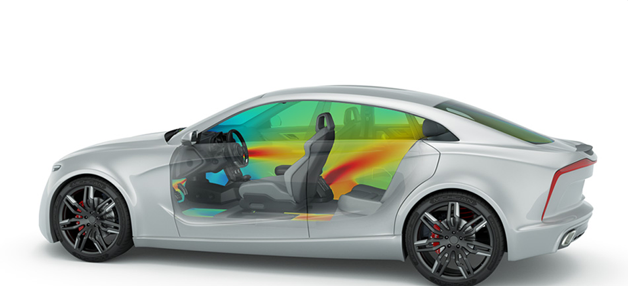
The use of aerodynamics in cars is a growing area of interest, especially with the global push for fuel efficiency and high-performance vehicles. In automotive engineering, aerodynamic simulation is used to reduce drag force and improve vehicle stability. For racing cars, an efficient car aerodynamics CFD design can lead to higher speeds and better cornering performance by generating downforce.

Every curve and vent in a modern car is influenced by CFD analysis of car aerodynamics. Engineers rely on aerodynamic simulation software to visualize airflow around the vehicle, making informed design decisions to reduce turbulence, enhance cooling, and lower fuel consumption. This integration of aerospace CFD simulation methods into the automotive industry showcases the crossover potential of aerodynamic cfd simulation technologies.

Figure 3- Flow around a Vehicle Aerodynamics CFD Simulation, ANSYS Fluent Aerodynamics Tutorial

Application of cfd in chemical engineering

Chemical engineering has a wide range of applications across various industries. Here are some of the most prominent ones:

• Energy industry: Chemical engineering is used to improve and refine fossil fuels and biogas. The final products have suitable characteristics for efficient energy production and also produce less pollution. CFD chemical engineering simulations are widely used to optimize and analyze energy industry projects.

• Food and beverage industry: Chemical engineering is used to produce food products, ensuring the quality and health of the products. For example, it is applied in the preparation of milk powder. Traditional methods of food production are often slow and require a significant amount of manpower.

• Water treatment: The treatment of water or sewage involves various steps and methods aimed at removing biological pollutants, such as bacteria, and separating unwanted salts and soil particles. To achieve these objectives, substances such as chlorine, which kills bacteria, and flocculants, which aggregate soil particles, are added to the water. CFD chemical engineering simulations are useful in the study of water treatment projects due to the capabilities of CFD in the analysis of multiphase systems.

Aerial view recirculation solid contact clarifier sedimentation tank, Water treatment solution, Industrial water treatment

Common Tools in Industrial Chemical Processes

In the following, some commonly used tools in industries to perform chemical reactions are introduced:

Fluidized bed reactors

In a fluidized bed, solid materials are placed in a tank as small particles. Gas or liquid enters the system from below, under pressure. This process causes the bed of solid materials to behave like a fluid physically. During this process, chemical reactions can occur between the entering fluid and the solid particles, facilitated by their extensive surface area. Additionally, the solid particles can be coated with another material, or they can be classified at different heights within the bed based on their size. fluidized bed CFD simulations are used for analysis and optimization of fluid dynamics and heat transfer within the reactor.

Mixing and stirred tank reactors

In mixing and stirred tank reactors, materials are blended using various methods, typically involving a rotating component such as a stirrer, to facilitate chemical reactions or achieve uniform mixtures. These materials can exist in solid, liquid, or gas phases. CFD simulations help in optimizing the mixing efficiency and understanding the flow patterns within the reactor for better reaction kinetics and heat transfer.

Heat exchanger

A heat exchanger is used to transfer heat from boilers to chemical reactants. These devices come in various types. Heat exchanger CFD simulations aid in designing heat exchangers with optimal heat transfer characteristics and minimal pressure drop, enhancing efficiency and performance.

Boiler

In boilers, the combustion process generates heat used for various purposes. This heat facilitates numerous chemical reactions within the boiler system. Moreover, the design of boilers exemplifies the principles of chemical engineering. CFD simulations are employed to optimize combustion efficiency, heat distribution, and pollutant emissions within the boiler chamber.

Pumps and compressors

Pumps and compressors are utilized to increase pressure and transfer fluids in industrial processes. CFD simulations are used to analyze fluid flow patterns, and pressure distribution, and optimize the performance and energy efficiency of pumps and compressors. CFD simulations assist in optimizing tray or packing design, vapor-liquid distribution, and overall column efficiency for improved separation performance.

Distillation columns

Distillation columns are used to separate fluid mixtures based on their boiling points. For instance, when oil enters a distillation column, its temperature is raised, causing a substantial portion to evaporate. As these materials ascend with the gas phase inside the column, their temperature decreases, leading to condensation. Different materials condense at various heights and temperatures within the column, thereby facilitating their separation based on boiling points.

A distillation column, Used for the separation of oil components

Simulation of Chemical Engineering Processes by ANSYS Fluent

ANSYS Fluet has many capabilities in chemical engineering CFD simulations. Among the capabilities of this software, the following features can be mentioned as CFD applications in chemical engineering:

• Mass transfer: ANSYS Fluent helps chemical engineers simulate key mass transfer processes like absorption and diffusion. It tracks how chemicals move in fluids, aiding in optimizing reaction and separation processes for efficient chemical production.

• Heat transfer: It is possible to simulate all three types of heat transfer, radiation, convection, and conduction, simultaneously in Fluent. By simulating the heat transfer processes in boilers, heat exchangers, and other equipment, chemical engineers can ensure and determine the desired temperature of the products. CFD chemical engineering simulations always include heat transfer calculations.

• Fluid flow: Fluent excels in its ability to simulate flow, accurately predicting pressure distributions and flow velocities. It effectively handles both laminar and turbulent flows, offering extensive capabilities for simulating turbulent phenomena. Moreover, Fluent supports the simulation of non-Newtonian fluids, further broadening its applicability in diverse industrial and engineering scenarios. Fluid flow simulation is based on fluid mechanics rules. Fluid mechanics for chemical engineers with microfluidics and CFD allows for precise modeling of complex fluid interactions, enhancing process optimization and innovation.

• Multiphase simulation: In all industrial chemical processes, multiphase flow is common. Fluent offers extensive capabilities for simulating multiphase flows, including scenarios where solid particles are suspended in fluids. The software can simulate the interaction between the fluid and the particles, the mutual interaction among the particles themselves, and the impact of particles on the fluid. This comprehensive approach allows for detailed analysis and optimization of processes involving complex multiphase phenomena. Multiphase simulation is the most important CFD application in chemical engineering.
  Mentioned simulation fields are common applications of CFD in chemical engineering.

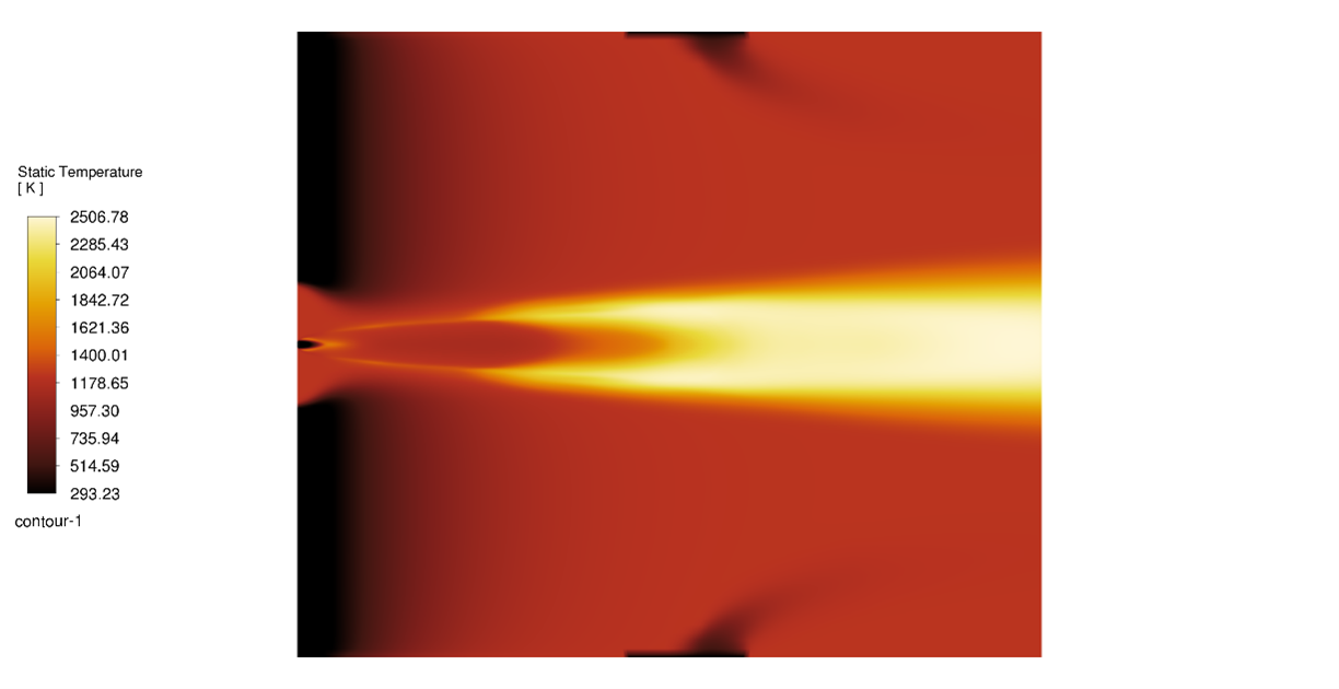
Static temperature contour, from “Methane-air Combustion Using GRI CHEMKIN Mechanism”

 Applications of Renewable Energy

Here are some common applications of renewable energy across various sectors:

Electricity Generation

Renewable energy is primarily used to generate electricity in a clean and sustainable manner. Technologies like solar panels, wind turbines, hydroelectric dams, and geothermal power plants convert natural forces into electrical energy without emitting greenhouse gases. This electricity powers residential homes, commercial buildings, and industrial facilities, helping to reduce reliance on fossil fuels and lowering carbon footprints globally.

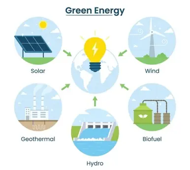
Figure 16- Electricity generation renewable source types

Heating and Cooling

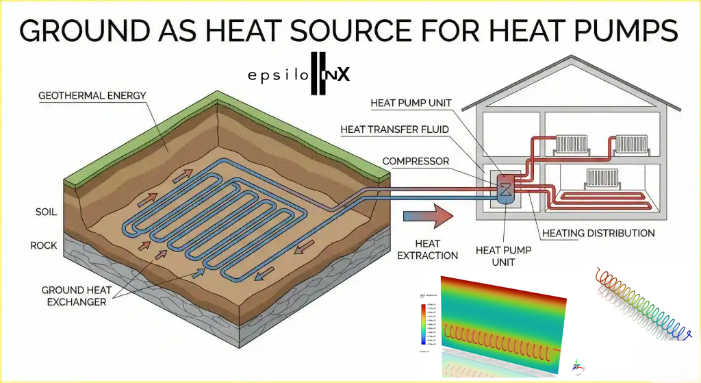
Renewable sources like geothermal energy and biomass provide effective heating and cooling solutions. Ground-source heat pumps use the Earth’s stable underground temperatures to heat or cool buildings efficiently, while biomass materials like wood chips and agricultural waste are burned or digested to produce heat for homes, greenhouses, and factories. These systems offer a low-emission alternative to conventional HVAC systems.

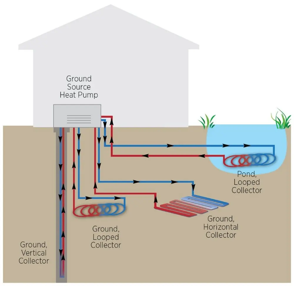
Figure 17- Geothermal Heat Pump Selection and Installation

Transportation

The transportation sector benefits from renewable energy through the use of biofuels and electric vehicles (EVs). Biofuels such as ethanol and biodiesel are derived from organic materials and can power cars, buses, and planes with lower emissions than traditional fuels. Additionally, EVs can be charged using electricity from renewable sources, making travel more environmentally friendly and reducing dependence on oil.

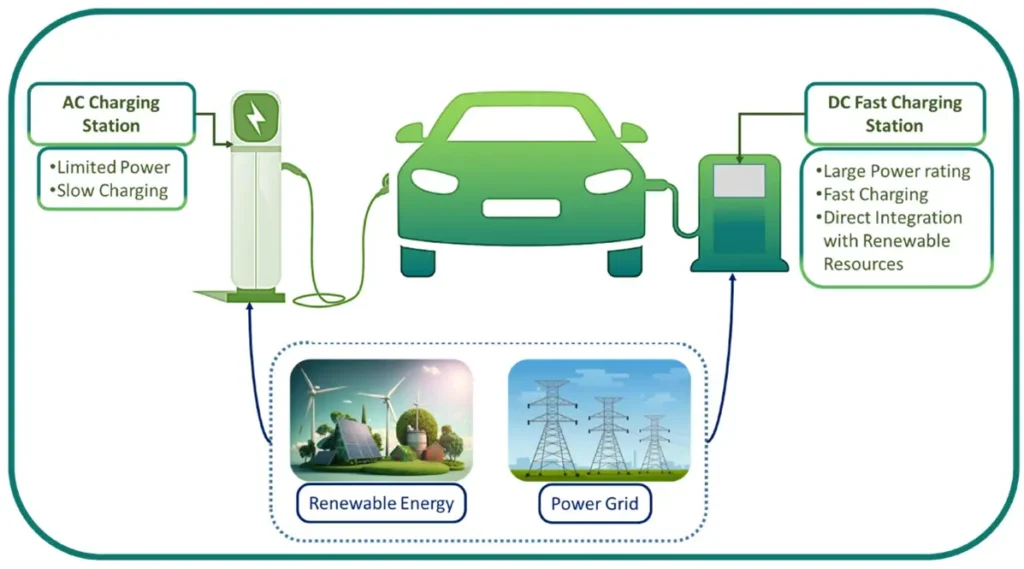
Figure 18- Sustainable Vehicles for Decarbonizing the Transport Sector

Water Desalination

Solar-powered desalination offers a sustainable solution to water scarcity, especially in arid and coastal regions. This process uses solar energy to power systems that remove salt from seawater, producing fresh drinking water. It is particularly valuable in off-grid or developing areas, where access to clean water is limited and conventional energy is costly or unavailable.

Agriculture

In agriculture, renewable energy supports sustainable farming practices. Solar panels are often used to power irrigation pumps, lighting, and small machinery in remote or off-grid farms. Biogas systems digest animal and crop waste to produce both electricity and natural fertilizer, promoting circular farming. These solutions reduce operating costs and environmental impact for farmers.

Figure 19- Solar Panels are Used to Power Irrigation Pumps, and Lighting

Industrial Processes

Industries are increasingly using renewable energy to power operations and reduce emissions. Renewable electricity from wind, solar, and hydro sources can run heavy machinery and manufacturing plants. Furthermore, green hydrogen produced through electrolysis with renewable power is becoming vital in high-temperature processes like steelmaking, offering a cleaner alternative to coal and gas.

Renewable Energy in Space Exploration

In the space industry, the transfer of fossil fuels is prohibitively expensive, and their frequent consumption presents logistical challenges. Renewable energy proves indispensable in space exploration and satellite technology, particularly through the utilization of solar energy and thermoelectric generators. These generators, functioning as semiconductors, produce electricity from temperature differentials. While their energy output is limited, they find essential applications in specialized sectors such as space industries.

Figure 20- Reaching for the Stars: How Solar Energy Empowers Space Exploration

Simulation of Renewable Energies by ANSYS Fluent

ANSYS Fluent is a powerful tool for CFD simulation for renewable energy systems, allowing engineers to analyze fluid flow and heat transfer processes critical to improving the performance of clean energy technologies. In wind turbine CFD simulation, Fluent helps model airflow dynamics, turbulence, and wake effects for blade optimization. In solar applications, solar panel CFD analysis and photovoltaic system thermal simulation enable users to study heat buildup and test cooling strategies such as air or liquid cooling, or even phase change materials. These simulations ensure higher efficiency and longer system lifespan.

Beyond solar and wind, Fluent is also widely used for geothermal energy CFD simulation, simulating subsurface fluid flow and heat extraction. It plays a key role in CFD simulation of solar thermal systems and energy storage units, helping design efficient thermal management systems. Overall, ANSYS Fluent renewable energy simulation enhances design accuracy, reduces prototyping costs, and supports CFD optimization of renewable energy systems. This leads to smarter, more reliable clean energy solutions tailored for real-world conditions.

Figure 21- CFD Simulation of Various Types of Renewable Energy Systems Using ANSYS Fluent by CFDLAND Experts

Sliding Mesh Applications

sliding mesh CFD simulation is used in various industries and engineering projects. Here are some common applications of sliding mesh:

Turbomachinery

In all turbomachines, the set of solid vanes move in a rotational manner; this movement may be to move the fluid, or the movement of the fluid causes the vanes to move. Examples include wind turbines, fans, and centrifugal pumps. With the movement of the solid body in the fluid, a sliding mesh is used for simulation. Usually, a cylindrical domain is considered around the blades, and the mesh inside this domain rotates with the blades. ANSYS Fluent CFD simulation is a very suitable option for designing and optimizing the turbomachine using the sliding mesh technique.

Sliding mesh can be used for the CFD simulation of wind turbines. The range within which the turbine blades rotate is considered the rotating domain.

Gear Pump

In a gear pump, two gears rotate close to each other to move the fluid flow. Sliding mesh can be used for the cylindrical domains in which each gear is placed. Engineers use sliding mesh CFD simulations in ANSYS Fluent to optimize and design gear pumps.

Generators and Electric Motors

There are rotating parts in generators and electric motors. Engineers use CFD simulations for heat transfer (thermal management) and to reduce the drag force of these rotating parts. In these simulations, sliding mesh is used for the domain containing the rotating part.

The part inside the electric motor rotates. CFD simulations can be used to reduce the drag force and check the heat transfer.

What is the difference between Dynamic mesh and Sliding mesh?

Choosing the right mesh technique depends on the complexity of your CFD simulation. Sliding Mesh is Ideal for scenarios with simple, predictable motions like rotation or translation. The computational efficiency comes from the cells simply sliding without changing shape. This makes it a preferred choice for applications like turbomachinery where, for example, turbine blades rotate at a constant speed.

Dynamic Mesh approach tackles complexities where the object’s movement is irregular, the domain size changes significantly, or the boundaries themselves move. Here, the mesh adapts to these changes, making it valuable for Fluid-Structure Interaction (FSI) simulations and piston engines where the domain experiences significant deformations.

Usually, dynamic mesh requires much more computing power than sliding mesh due to the changing shape of the cells and the need for mesh regeneration.

Simulation of Sliding Mesh by ANSYS Fluent

In ANSYS Fluent, fixed and moving domains are defined initially, followed by mesh generation. Along the border between these domains, it is crucial to ensure a high-quality mesh, with cells near the interface being uniformly sized. Once the mesh is created, Fluent settings dictate which domain remains fixed and which one moves. Fluent effectively connects cells on both sides of the interface, solving equations for heat transfer, Navier-Stokes turbulence, and other relevant physics. Results from cells on one side of the interface are transferred to the other side, facilitating accurate simulation of fluid flow and interaction between stationary and moving components.

ANSYS Fluent has been extensively used in numerous turbomachinery simulation projects. The CFD simulations conducted with this software have yielded highly effective results, enabling the efficient design of turbines and pumps using sliding mesh techniques. These successes have significantly contributed to ANSYS Fluent’s popularity as a preferred CFD simulation software among engineers. It is recommended to perform sliding mesh CFD simulation with ANSYS Fluent.

Velocity contour, adopted from “Vertical Axis Wind Turbine With Guide Vane CFD Simulation”

What Exactly Are Acoustics and Aeroacoustics?

When we hear the word “sound,” we often think about music, voices, or even noises around us. But for engineers, sound is much more than that. It is a science that helps us understand how sound is created, how it travels, and how it is heard. This science is called acoustics, and it plays a very important role in designing quieter machines, safer workplaces, and more comfortable spaces.

Acoustics is the study of sound waves. A sound wave is created when an object vibrates, like the strings of a guitar or the engine of a car. These vibrations cause changes in air pressure, which we hear as sound. Acoustics focuses on how these sound waves move through different mediums, such as air, water, or solid materials. It also looks at how sound waves behave—how they reflect, absorb, or travel to reach our ears. In engineering, acoustics helps us solve problems like reducing noise in factories, improving music quality in concert halls, and controlling sound in offices or homes.

Figure 1: Visualizing the sources of sound in engineering acoustics. The field of Acoustics (left) often studies sound originating from structural vibration. In contrast, Aeroacoustics (right) focuses on sound generated directly by turbulent fluid flow.

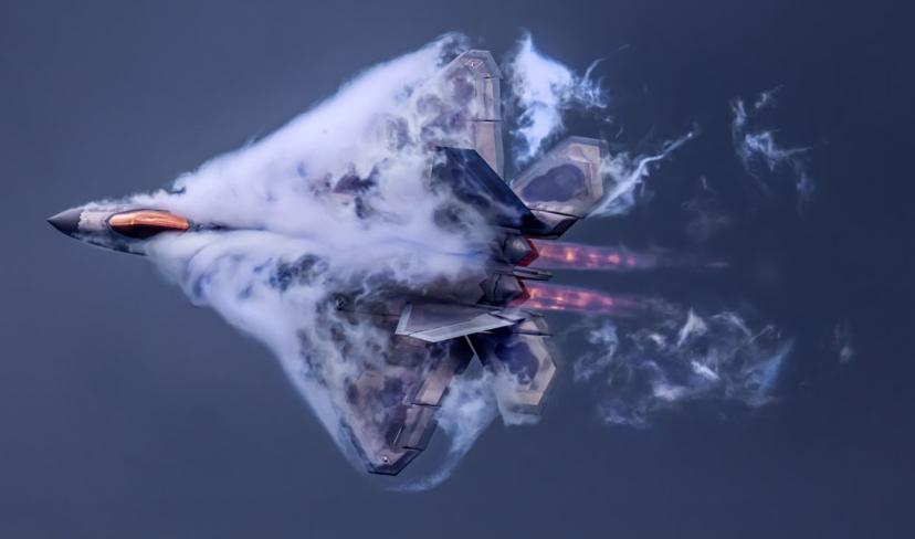
On the other hand, aeroacoustics is a special branch of acoustics. It focuses on sound that is created by moving fluids like air or water. For example, the noise made by an airplane flying through the sky, the hum of a fan, or the sound of air rushing through a ventilation system are all examples of aeroacoustics. In these cases, the sound does not come from vibrations of solid objects. Instead, it comes from the movement of fluids and the turbulence they create. Engineers use aeroacoustics to study how air or water flows and how this movement creates sound. This helps them design quieter airplanes, better wind turbines, and more efficient ventilation systems. Both acoustics and aeroacoustics are important sciences that help engineers predict and control sound. Whether it is reducing noise pollution in cities or designing quieter machines, these fields are key to improving the way we live and work.

Core Concepts in Acoustics and Aeroacoustics

Acoustics is all about understanding how sound behaves. One of the most important concepts in acoustics is pressure fluctuation. Sound waves are actually changes in pressure that travel through air, water, or solid objects. Imagine dropping a pebble into water. The ripples spreading out are like the sound waves created by pressure changes. These waves have areas of high pressure (compression) and low pressure (rarefaction). This movement of pressure is what allows sound to travel from its source to the listener.

In engineering, pressure fluctuations are key to understanding how sound propagates, or moves, from one place to another. For example, in a factory filled with noisy machines, the sound travels through the air as pressure waves. Engineers study these waves to find ways to reduce noise levels. They may use materials that absorb sound or design machines that vibrate less. This is called industrial noise control, and it’s important for keeping workers safe and productive.

Figure 2: A visual bridge between aeroacoustics and musical acoustics, illustrating how the same physical principles of air movement and pressure waves govern both the roar of aircraft and the resonance of a guitar.

Aeroacoustics is the study of how sound is created by moving fluids, such as air or water. It links fluid dynamics—the study of how fluids move—with sound generation. This field helps engineers understand why noise is produced and how it can be controlled. For example, when air flows quickly over the wings of an airplane or through a ventilation duct, it creates turbulence. This turbulence leads to changes in pressure, which generate sound. The sound caused by moving fluids is called aeroacoustics noise.

One key part of aeroacoustics is fluid flow acoustics. This focuses on how the movement of air or water produces sound. For example:

• Aircraft noise: Fast-moving air interacts with airplane wings and engines, creating turbulence and noise. This is a major challenge for engineers working to reduce noise near airports.

• Ventilation systems: When air moves through ducts and interacts with fans, it can cause vibrations and turbulence, leading to unwanted noise in buildings.

• Wind turbine noise: The spinning blades of wind turbines create airflow patterns that produce sound. Engineers study these flows to design quieter turbines, especially for areas near residential zones.

Porous media application

are materials that contain a network of interconnected pores or voids, allowing fluids to pass through them (Fig.1). Examples include soil, foam, filters, and biological tissues. From a fluid dynamics perspective, understanding fluid flow in porous media is essential for analyzing systems involving filtration, heat transfer, and chemical processing. Whether you’re new to the topic or looking to deepen your understanding, our website, CFDLAND, offers helpful porous media fluent tutorial and examples to guide you through the practical aspects of working with porous media in ANSYS Fluent and other CFD approaches. The porous media meaning in CFD context refers to regions in your model that introduce resistance to fluid flow—often needing special treatment in simulations like porous media fluent models.

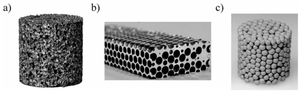
Figure 1- Different types of porous materials: a) closed-cell metal foam; b) hollow alumina spheres embedded in a magnesium matrix c) hollow sphere foam Fe0.88 Cr0.12 [1]

Porous Media Meaning

In materials science, a porous medium or a porous material is a material containing pores (voids). A fluid-saturated porous media consists of a matrix and a porous space, with the latter usually interconnected and filled by a fluid (effective porosity). The matrix is composed of solid material as well as some occluded porosity which is not an effective porosity and it may be saturated with fluid. In another approach, a porous medium is a combination of two continua, i.e. the skeleton continuum and the fluid continuum (Figure 2.1). The skeleton is composed of the matrix and connected porous space without any fluid, whereas the fluid continuum contains saturated porous space with fluid without any matrix.

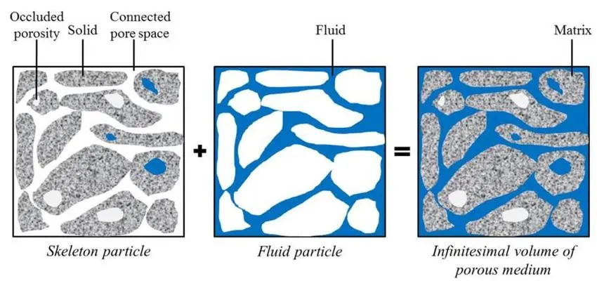
Figure 2- Porous medium as the superposition of skeleton particle and fluid particle in an infinitesimal volume[2]

Physical Characteristics of Porous Media

Let’s explore the physical characteristics that make fluid flow in a porous media a fundamental aspect of many disciplines, highlighting the importance of porous media flow and the detailed analysis of flow in a porous media.

Porosity

Porosity is the ratio of void volume to the total volume of a porous medium. The Fig.3 shows four cylindrical samples with different levels of porosity, ranging from 64% (most porous) to dense (no visible pores). The samples illustrate how increasing porosity results in more open structure, while the dense sample has a solid structure with minimal or no pores.

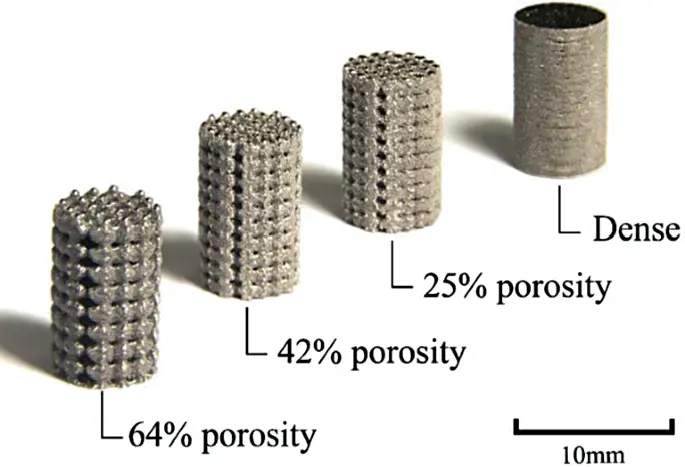
Figure 3- porous media filter: solid and porous Ti-Ta cylinders [3]

Permeability

The ability of a porous material to transmit fluids. It is a key property that determines how easily fluids can flow through the medium. Fig.4 shows how permeability decreases from gravel to clay, as water flows quickly through gravel but takes much longer to pass through sand, silt, and especially clay.

Figure 4- Permeability of different soil types: water flow rates through gravel, sand, silt, and clay

Tortuosity

Tortuosity is a measure of the complexity or lengthening of the flow path a fluid takes through a porous medium compared to the straight-line distance (Fig.5).

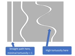
Figure 5- Comparison of Straight and Tortuous Flow Paths in Porous Media

Capillary Action

Capillary action is another remarkable physical characteristic seen in porous media, where fluid movement occurs against the force of gravity due to surface tension effects (Fig.6).

Figure 6- Effect of particle size and pore radius on capillary rise in porous media

Porous Media Equations

When analyzing fluid flow in a porous media, several key equations are used to model the movement of fluids through materials with internal voids. Moreover, the relationship between flow rate and pressure difference can be changeable for porous media flow. As shown in the Fig.7, the first part of the curve from the origin shows that the relationship is linear. When the flow rate is large, the non-linear relationship starts to show up.

Figure 7- Relationship between flow rate and pressure difference

The two primary equations often used in porous media modeling are Darcy’s Law and the Forchheimer equation, each addressing different flow conditions.

Darcy’s Law

For slow, steady flows where inertial effects are negligible, Darcy’s Law is commonly used to describe the fluid velocity (𝑣) in porous media. The equation is:

here, 𝑣 is fluid velocity, 𝐾 is permeability of the porous medium, 𝜇 is dynamic viscosity, and ∇𝑃 is pressure gradient. This simple yet fundamental relationship indicates that the flow rate is proportional to the pressure difference and the permeability of the material. It’s widely used in ANSYS Fluent porous media simulations when the flow is considered laminar and slow.

Forchheimer Equation

For higher velocities, where inertial effects become important, Darcy’s Law needs to be adjusted. The Forchheimer equation includes a correction term for inertial resistance:

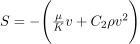
here, 𝑆 is momentum sink/source term, 𝐶2 is inertial resistance coefficient, 𝜌 is fluid density and 𝑣 is fluid velocity. This extended equation is used when the flow through the porous media becomes turbulent or faster, and it’s essential for modeling more complex systems like those found in porous media ANSYS Fluent simulations.

Energy Equation

In many cases, heat transfer is also a critical part of porous media flow. The energy equation in porous media is similar to the standard heat transfer equation, but it includes the effects of the porous structure:

here, 𝑇 is temperature, 𝑘𝑒𝑓𝑓 is effective thermal conductivity and 𝑄 is volumetric heat source. This equation helps model fluid flow and heat transfer in porous medium, allowing engineers to predict temperature distributions within porous materials.

Governing equations

The governing equations for the steady flow are as follows:

where u = [u, v, w] T is the velocity vector, p is the pressure, ν is the kinematic viscosity and ρ is density. Sporous is the source term due to the presence of the porous media, and is only considered when using the porous media model. ANSYS Fluent uses the generalized formula to model porous media, as detailed in Fluent user manual (ANSYS Fluent User Guide, Release 15.0). The porous media model in ANSYS uses a superficial velocity inside the porous media instead of the actual velocity in the media. Thus, the model cannot predict the real velocity inside the media. However, it produces results for the pressure drop and velocity values. The modeling for the porous media uses the sink term Sporous, which is defined as follows ANSYS Inc (2013):

where D is the matrix of viscous resistance coefficients, which is a diagonal matrix containing the resistance coefficient corresponding to each direction. C is the matrix of inertial resistance coefficients, which has a diagonal form similar to the matrix D. The terms appearing in this equation called Darcy and Forchheimer drag terms.

ANSYS Fluent Porous Media Simulation

Porous media modeling involves representing fluid flow and sometimes heat transfer through a solid matrix containing interconnected voids. In CFD, this complex behavior can be effectively simulated using ANSYS Fluent, a powerful tool for Porous Media CFD applications. Fluids can move easily within a layer of the shale, but cannot move across layers (Fig.8).

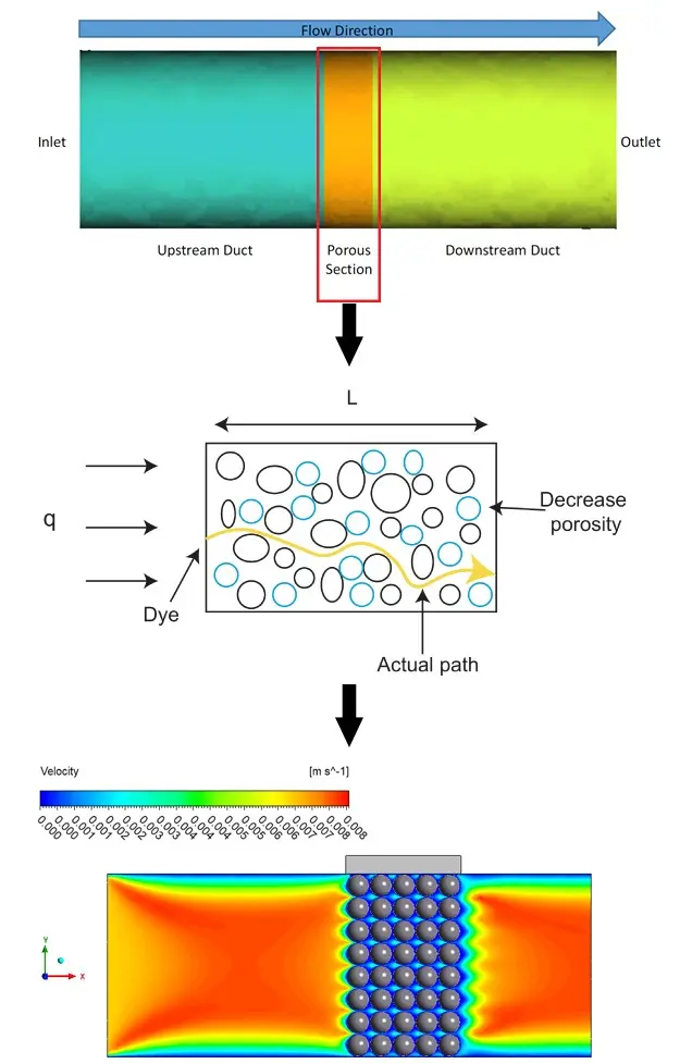
Figure 8- Example of fluid flow in a porous medium

Turbulence

is a complex and fluctuating flow phenomenon commonly encountered in real-life and engineering applications. Despite decades of research, its underlying physics remains only partially understood, and no general analytical solution exists for most turbulent flows. As a result, computational fluid dynamics (CFD) relies on turbulence models—mathematical approximations that predict the statistical behavior of turbulence—especially when direct numerical simulation is impractical. These models are essential for estimating key effects like wall shear stress and energy dissipation, allowing engineers to analyze and design systems exposed to turbulent conditions. In terms of engineering applications, the turbulent regime occurs in the aerodynamics of all vehicles such as cars, planes, and ships; but also in many industrial applications such as heat exchangers, quenching processes, or continuous casting of steel.

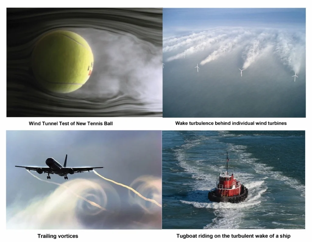
Figure 1- Examples of turbulent dynamics in in real-life and engineering applications

Flow Regime Classification in Fluid Mechanics

If you turn on a faucet (that doesn’t have an aerator or other attachment) at a very low flow rate the water will flow out very smoothly—almost “glass-like.” If you increase the flow rate, the water will exit in a churned-up, chaotic manner (Fig.2). These are examples of how a viscous flow can be laminar or turbulent, respectively. A laminar flow is one in which the fluid particles move in smooth layers, or laminas; a turbulent flow is one in which the fluid particles rapidly mix as they move along due to random three dimensional velocity fluctuations.

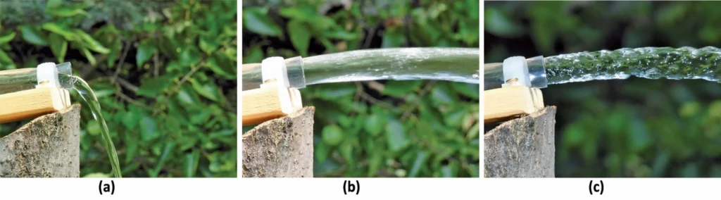
Figure 2- Water exiting a tube: (a) laminar flow at low flow rate, (b) turbulent flow at high flow rate, and (c) same as (b) but with a short shutter exposure to capture individual eddies.

Reynolds Number

The transition from laminar to turbulent flow depends on below parameters among other things.

1. Geometry,

2. Surface roughness,

3. Flow velocity,

4. Surface temperature,

5. Type of fluid.

A flow that alternates between being laminar and turbulent is called transitional. The experiments conducted by Osborne Reynolds in the 1880s resulted in the establishment of the dimensionless Reynolds number, Re, as the key parameter for the determination of the flow regime in pipes. Osborne Reynolds built 6-ft. long glass tubes with diameters of 2.68, 1.53, and 0.789 cm with trumpet mouths and passed water through them (Fig.3).

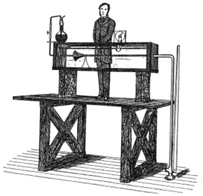
Figure 3- Osborne Reynolds’ original apparatus for demonstrating the onset of turbulence in pipes.

He found that at a low flow rate and/or with a small diameter tube, an injected color streak is seen as a steady streak (Fig.4).

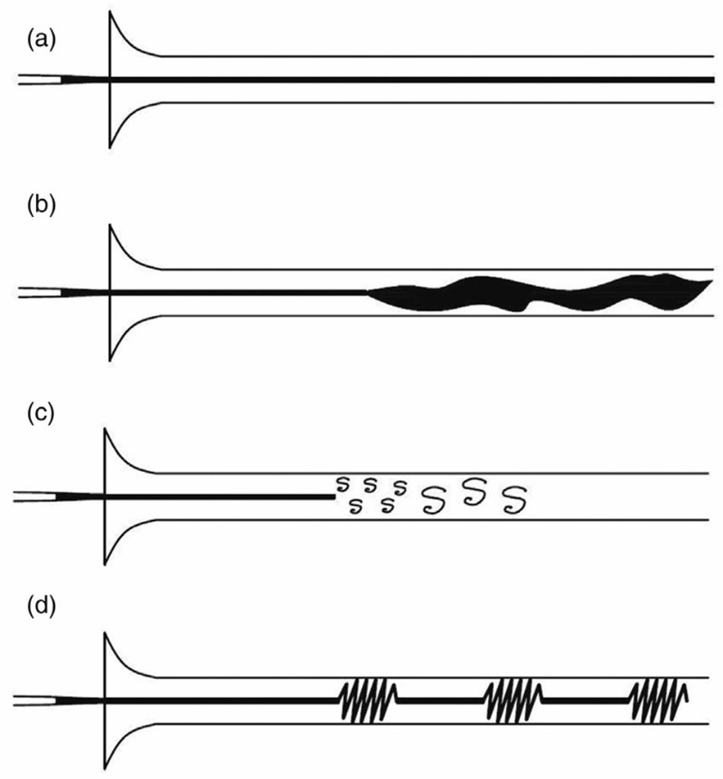
Figure 4- Osborne Reynolds’ experiment on laminar to turbulent flow in a pipe.

In other words, the flow is laminar at low Re where small perturbations are damped out by viscosity. Note that a laminar flow in a smooth long pipe in Fig. 4(a) is named after Poiseuille. At a higher flow rate, the color band shown in Fig. 4 (b) appears to expand and mix with the water. When viewing the tube by the light of an electric spark (Fig. 4 (c)), the mass of color resolves itself into a mass of more or less distinct curls, in which eddies can be seen. In the transitional realm of an intermediate flow rate, as depicted by Fig.4 (d), we see the intermittent character of the flow motion caused by the disturbances, which appear as flashes succeeding each other inside the tube. In other words, we see sporadic bursts of turbulence alternating with laminar flow, indicating a problem with multiple solutions. Consequently, some have approached the origin of turbulence via the bifurcation/chaos method.

After exhaustive experiments in the 1880s, Osborne Reynolds discovered that the flow regime depends mainly on the ratio of inertial forces to viscous forces in the fluid. This ratio is called the Reynolds number and is expressed for internal flow in a circular pipe as shown in the Fig.5.

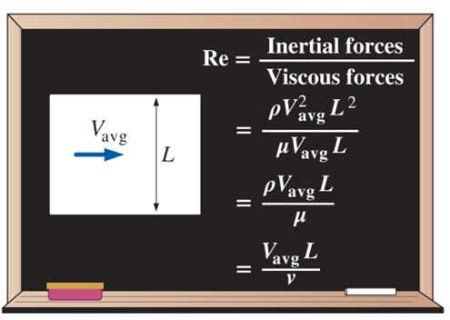
Figure 5- The Reynolds number can be viewed as the ratio of inertial forces to viscous forces acting on a fluid element.

where Vavg = average flow velocity (m/s), D = characteristic length of the geometry (diameter in this case, in m), and 𝜈 = 𝜇/𝜌 = kinematic viscosity of the fluid (m2/s). Note that the Reynolds number is a dimensionless quantity. Also, kinematic viscosity has units m2/s, and can be viewed as viscous diffusivity or diffusivity for momentum.

Flow Regimes for Common Geometrical Configurations

In fluid mechanics, flow behavior significantly depends on the geometry of the object around or through which the fluid moves. Each geometry leads to unique interactions between the fluid and the surface, and thus influences the transition between laminar, transitional, and turbulent flow regimes. These regimes are primarily classified based on the Reynolds number, a dimensionless value that captures the balance between inertial and viscous forces in a flow. Table1 summarizes the typical flow regimes for several common geometries encountered in engineering applications. This classification helps engineers select proper turbulence models in CFD simulations (like in ANSYS Fluent) and optimize mesh quality based on the expected flow behavior.

Table 1- Flow Regimes for Common Geometrical Configurations

Flow Regimes in Free Convection

In free (natural) convection, the flow regime is determined primarily by the Rayleigh number (Ra), which combines the effects of buoyancy (via the Grashof number) and thermal diffusivity (via the Prandtl number). Unlike forced convection, where the Reynolds number governs flow behavior, free convection relies on Ra to indicate whether the flow is laminar, transitional, or turbulent.

​

​

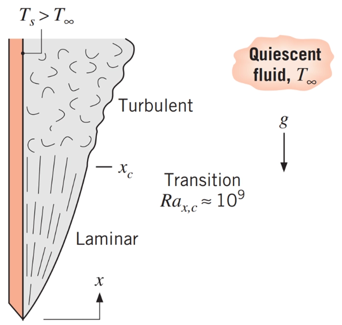
Figure 6- Free convection boundary layer transition on a vertical plate.

Table 2- Flow Regimes in Natural Convection Based on Rayleigh Number

Key Takeaways:

1. The critical Reynolds number varies with geometry and surface conditions.

2. Transition from laminar to turbulent flow is gradual and can be affected by surface roughness, flow disturbances, and inlet conditions.

3. For external geometries, boundary layer behavior plays a major role in determining drag and separation.

Turbulent Flows Characteristics

Because of the complex nature of turbulence, providing a precise definition is often ineffective. Instead, it is more practical to describe turbulence through its key characteristics. In their book “A First Course in Turbulence”, Tennekes and Lumley outline several defining features of turbulent flow, including:

1. Irregularity

2. High diffusivity

3. Occurrence at high Reynolds numbers

4. Fluctuating three-dimensional vorticity

5. Energy dissipation

6. Behavior consistent with the continuum assumption

7. A property of the flow, not the fluid itself

These traits collectively capture the essential nature of turbulent motion.

Irregularity

Turbulent flows are inherently irregular and chaotic, exhibiting complex, unpredictable patterns that vary in space and time. This randomness makes a fully deterministic or exact prediction nearly impossible. As a result, turbulence is often studied using statistical or averaged methods.

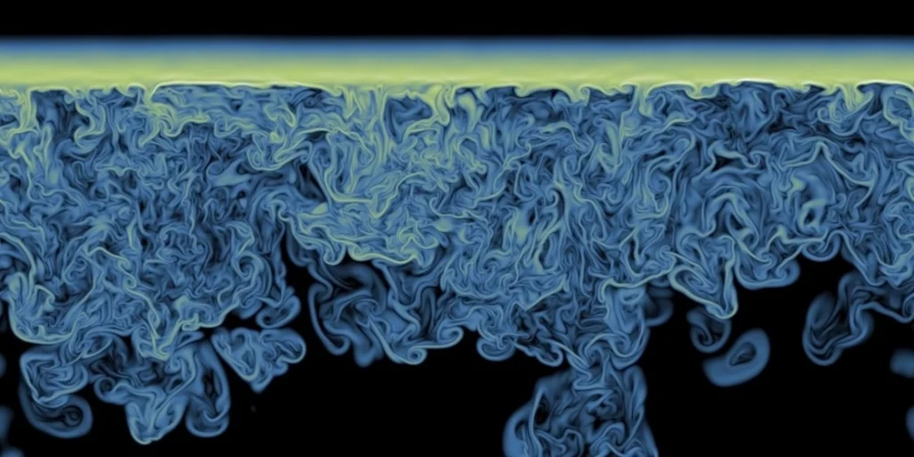
Figure 7- irregularity: a characteristic of turbulent flows.

Diffusivity

 Turbulence significantly enhances the mixing and transport of momentum, heat, and mass. The chaotic eddies promote rapid diffusion across the flow, making turbulent flows far more effective at mixing than laminar ones. If a seemingly random flow does not demonstrate this enhanced mixing, it cannot truly be classified as turbulent.

Figure 8- Diffusivity of Turbulence Lead to Mix Layers

Large Reynolds number

Turbulence typically arises in flows with high Reynolds numbers, where inertial forces dominate over viscous forces. It results from the intricate interplay between non-linear convective effects and viscous dissipation in the Navier–Stokes equations. This interaction leads to instability and ultimately a transition from laminar to turbulent motion.

Figure 9- High Reynolds Number Flow Example

Three-Dimensional vorticity fluctuations.

Turbulent flows are fundamentally three-dimensional and rotational, meaning they contain continuously fluctuating vorticity in all directions. These swirling motions are sustained through mechanisms such as vortex stretching, which cannot occur in purely two-dimensional flows.

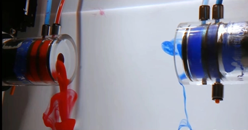
Figure 10- 3D Vorticity Turbulence Structures

Dissipation

Turbulence is dissipative by nature. The kinetic energy introduced at larger scales cascades down to smaller scales, where it is eventually transformed into thermal energy due to viscous effects. Without continuous energy input, turbulent flows gradually decay and revert to a more ordered state.

Figure 11- Energy Dissipation in Turbulence Flow of Water Waves

Continuum

Despite the small-scale structures in turbulence, the flow remains within the continuum regime. Even the tiniest turbulent eddies are much larger than molecular dimensions, allowing classical fluid dynamics to model the behavior effectively using continuum-based equations.

Figure 12- Continuum Assumption in Turbulent Flow in the nature

Feature of a flow, not fluid

Turbulence is not an intrinsic property of the fluid but rather a behavior exhibited by the flow under certain conditions—particularly at high Reynolds numbers. Different fluids may behave similarly under turbulent conditions, highlighting that turbulence depends on flow configuration, not fluid identity.

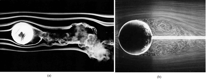
Figure 13- (a) Air flow over a spinning baseball, (b) Water flow over a sphere.

Turbulence Modeling Equations

Both laminar and turbulent flows satisfy the continuity and momentum equations are to be solved for velocity and pressure.

For laminar flow, where there are no random fluctuations, we go right to the attack and solve them for a variety of geometries. For turbulent flow, because of the fluctuations, every velocity and pressure term in equations (1) is a rapidly varying random function of time and space. At present our mathematics cannot handle such instantaneous fluctuating variables. No single pair of random functions V(x, y, z, t) and p(x, y, z, t) is known to be a solution to equations (1). Moreover, our attention as engineers is toward the average or mean values of velocity, pressure, shear stress, and the like in a high-Reynolds-number (turbulent) flow. This approach led Osborne Reynolds in 1895 to rewrite equations (1) in terms of mean or time-averaged turbulent variables. The time mean of a turbulent function u(x, y, z, t) is defined by:

where T is an averaging period taken to be longer than any significant period of the fluctuations themselves. The mean values of turbulent velocity and pressure are illustrated in Fig. 14. For turbulent gas and water flows, an averaging period T=5 s is usually quite adequate.

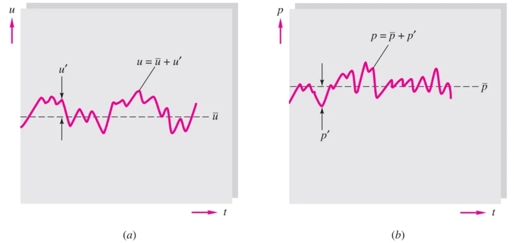
Figure 14- Definition of mean and fluctuating turbulent variables: (a) velocity; (b) pressure.

The fluctuation u′ is defined as the deviation of u from its average value

also shown in Fig. 14. It follows by definition that a fluctuation has zero mean value:

However, the mean square of a fluctuation is not zero and is a measure of the intensity of the turbulence:

Nor in general are the mean fluctuation products such as  and zero in a typical turbulent flow. Reynolds’ idea was to split each property into mean plus fluctuating variables:

Substitute these into Eqs. (1), and take the time mean of each equation. The continuity relation reduces to

which is no different from a laminar continuity relation. However, each component of the momentum equation (1), after time averaging, will contain mean values plus three mean products, or correlations, of fluctuating velocities. The most important of these is the momentum relation in the mainstream, or x, direction, which takes the form

The three correlation terms [latex]−ρu′2,−ρu′v′,−ρu′w′[/latex],  are called turbulent stresses because they have the same dimensions and occur right alongside the newtonian (laminar) stress terms and so on. Actually, they are convective acceleration terms (which is why the density appears), not stresses, but they have the mathematical effect of stress and are so termed almost universally in the literature.

Vorticity, Vortex, and Eddies in Fluid Dynamics

In fluid dynamics, rotational motion plays a fundamental role in shaping how fluids behave under various conditions. Key concepts such as vorticity, vortex, and eddies help us describe and understand different aspects of rotational behavior in flows. While these terms are closely related, each has a distinct meaning and function—vorticity is a mathematical measure of local rotation, a vortex is a physical region where fluid rotates coherently, and eddies are localized swirling motions that often drive mixing. This article explores their definitions, differences, and how they appear in both laminar and turbulent flows.

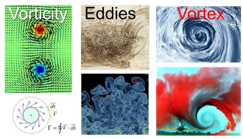
Figure 15- Vorticity, Vortex, and Eddies in Fluid Dynamics